SCM Automation, Part 2: From Backward Planning to Feasible Schedules

SCM automation: 1. Delivery promises · 2. Feasible scheduling · 3. Accountable automation.

“If the customer needs the windows next Friday, when must we start?” is a reasonable planning question. Its apparent simplicity conceals several different calculations.

We need a deadline for ordering materials, a feasible allocation of production resources, a release decision for the shop floor and a realistic forecast of customer receipt. A single subtraction cannot answer all four.

The KMS ITC position is that a useful schedule must explain both its feasibility and the conditions under which it stops being feasible. The objective is to expose actionable constraints early enough for the business to respond. A detailed Gantt chart is useful only to the extent that it represents those constraints faithfully.

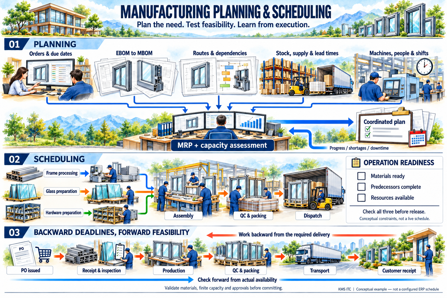
English adaptation of the supplied manufacturing panorama. Read it in three layers: planning establishes requirements; scheduling coordinates operations; backward deadlines are tested against actual availability. EBOM and MBOM mean engineering and manufacturing bills of materials. This is a conceptual illustration, not a live schedule or verified Pronto configuration. Open the full-size infographic.

Separate direction, constraints and policy

Backward scheduling starts from a required completion date to calculate a latest start. Forward scheduling starts from an available date to calculate an earliest finish. Microsoft documents both directions for production scheduling. Neither direction alone establishes whether a schedule respects physical limits. Microsoft Learn: Operations scheduling.

Four independent choices should be visible in a scheduling design:

Design choice	What it determines
Direction	Whether calculation starts from a required finish or an available start
Constraint model	Which material, resource, calendar and dependency restrictions are enforced
Objective and sequencing	How feasible alternatives balance delivery, setup, cost and priority
Release and revision policy	When work becomes executable and how changes are authorised

Backward scheduling can include finite capacity. Microsoft’s Planning Optimization documentation explicitly describes backward scheduling of planned production orders that takes existing resource reservations into account when the relevant finite-capacity settings are enabled. Finite-capacity behaviour also depends on the configured time fence. Microsoft Learn: Finite capacity planning and scheduling.

Our practical workflow is to calculate deadlines from demand, evaluate feasibility against current constraints, compare recovery options when necessary, and calculate the resulting delivery outcome from the available state. A suitable engine may perform several of these steps together. This is a decision workflow, not a requirement to run two separate algorithms or a description of Pronto configuration.

The eleven-day example is an action deadline

Suppose customer receipt is required at instant T. For this first example only, assume one common working calendar, wholly serial activities, fixed durations, immediate hand-offs, and no competing work, holidays, queues, failures or buffers. The purchase lead time starts when an approved PO is issued and ends when goods reach the factory. Approval time is excluded.

Milestone	Duration until the next milestone	Latest instant
Approved PO issued	5 working days of supply lead time	T−11
Material arrives; receiving inspection starts	1 working day	T−6
Production starts	3 working days	T−5
QC and packing start	1 working day	T−2
Dispatch; transport starts	1 working day	T−1
Customer receipt	—	T

The arithmetic is 5 + 1 + 3 + 1 + 1 = 11 working days. Under these assumptions, issue the approved PO no later than T−11. If approval requires another two working days before issue, its latest start is T−13.

This establishes when an action must occur under the model. It does not show that the supplier accepts the date, that production capacity exists, or that transport and receiving windows align. If today is already later than T−11, the baseline assumption set is no longer sufficient; investigate which dependency can actually change.

Keep milestones defined as instants and map them to actual calendars before quoting dates. “Five days” can otherwise conceal different supplier workweeks, shift boundaries, dispatch cut-offs and customer receiving hours. Count receiving inspection once: if a purchased lead-time field already includes it, adding it again would overstate the requirement.

Model the operation network before calculating the total

In a configurable window, the frame, glass and hardware can follow separate paths before assembly. Summing all three path durations would treat parallel work as serial. Treating them as independent without checking shared equipment or people would make the opposite error.

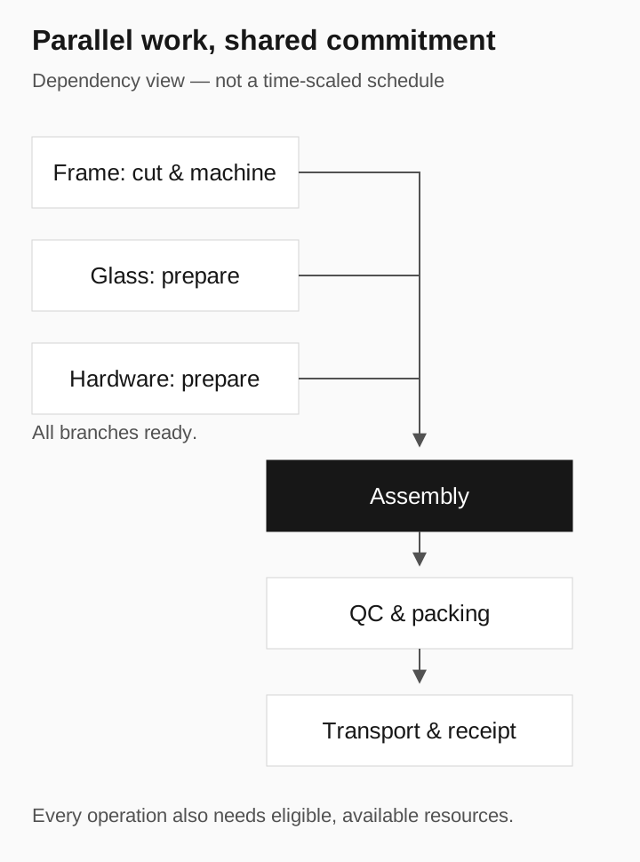
Conceptual dependency graph. Branches may overlap only where their resources permit. The drawing is neither a time-scaled Gantt chart nor a configured ERP routing.

Consider a second, independent worked example. Use abstract working-day boundaries measured from day 0, one common calendar, no uncertainty and distinct resources unless stated otherwise:

• The frame is ready at day 4, after cutting and machining.
• Glass is ready at day 6, including its required preparation and inspection.
• Hardware is ready at day 2.
• Assembly takes 2 days, QC and packing 1 day, and transport 1 day.

With assembly capacity available from day 6, assembly starts at max(4, 6, 2) = 6. It finishes at day 8; QC and packing finish at day 9; customer receipt is day 10. The path to receipt is 10 days, not the sum of all three upstream branches and downstream durations.

Now suppose the only eligible assembly cell is occupied until day 8, then has an uninterrupted two-day slot. Assembly starts at day 8 and receipt moves to day 12. Expediting glass from day 6 to day 5 produces no delivery improvement in this scenario: assembly remains the controlling constraint.

This illustrates why recovery actions should be evaluated by their effect on the customer outcome. The component attracting the most attention is not necessarily the dependency controlling completion.

A documented parallel branch on an automotive assembly line

Toyota’s virtual plant tour describes removing vehicle doors, installing glass and other parts on a separate door assembly line, then reattaching the doors later. This is a concrete example of a branch leaving and rejoining the main production flow. Toyota: Car Production Process — Assembly.

The transferable modelling principle is the join condition. In our analysis, a branch has to return with the correct item, configuration and quality status at the required point in the main flow. Treating a finished subassembly as an anonymous unit can hide a sequencing problem even when its quantity is correct. We are applying that principle to the window example; we are not claiming to know Toyota’s internal scheduling rules or detailed cycle times.

Readiness is a lower bound, not a booked start

For an operation, the later of predecessor completion and usable material availability establishes an earliest readiness time. A scheduling engine must then find a compatible resource allocation on or after that boundary.

For assembly requiring a machine, a qualified operator and a fixture together, the allocation must cover their required concurrent intervals. The earliest free instant on each separate calendar is insufficient if the required overlap does not last long enough. If the process permits an unattended machine cycle, the labour interval may be shorter; the model should reflect the actual operation.

A compact specification is:

1. Establish operation readiness from dependencies and usable materials.
2. Identify resources qualified for the operation and product revision.
3. Find calendar intervals with enough simultaneous capacity for the required durations.
4. Apply setup, transfer, batch and splitting rules supported by the process.
5. Reserve the selected allocation and propagate completion to successors.

Microsoft’s job-scheduling documentation separates detailed job start/end times, resource selection, finite capacity and finite material availability. Its finite-material behaviour checks materials for the operation start; this is more precise than assuming every component must arrive before the first production operation. Microsoft Learn: Job scheduling.

In our example, glass required at assembly need not necessarily arrive before frame cutting. However, an operation-level material model must preserve the right component specification, quantity, allocation and quality status. “In stock somewhere” is not equivalent to “usable here for this order”.

Capability establishes eligibility; capacity establishes availability

A routing that always names Machine 7 can obscure useful alternatives. A routing expressed in required capabilities can allow a qualified resource to be selected later.

Microsoft’s capability-based scheduling page describes requirements matched to resource capabilities, including effective dates and proficiency levels. Crucially, that particular page describes resource selection during infinite-capacity scheduling. It should not be read as evidence that capability matching itself prevents overload, or that every finite-capacity engine supports the same combination of features. Microsoft Learn: Scheduling with resource selection based on capability.

For architecture and acceptance testing, maintain three separate checks:

Eligibility: Can this combination of machine, tooling and people make this product to the required specification?

Availability: Are the necessary resources simultaneously usable for the required interval, after accounting for calendars and reservations?

Authority: Is this alternative route or subcontractor approved for this order and quality requirement?

The third check is easily missed. A technically capable alternative can require process qualification or customer acceptance. A scheduling recommendation should expose those prerequisites before anyone treats the alternative as executable capacity.

Optimisation needs a stated business objective

The basic job-shop problem already involves precedence and machine exclusivity constraints. Google’s OR-Tools example demonstrates these constraints while minimising makespan, the overall time needed to finish the modelled jobs. Google for Developers: The Job Shop Problem.

A commercial factory may need a different objective. Minimising makespan can be a poor proxy when one customer has a narrow installation window and another can accept delivery later. Reducing setups can be valuable, but a large batch may delay several urgent orders.

Our recommendation is to agree the ranking of outcomes before tuning the optimiser. Keep mandatory safety and quality constraints hard. Represent acceptable commercial compromises explicitly, such as overtime, approved subcontracting, split deliveries or lateness with an identified cost. Use a hierarchy of objectives where a weighted sum would conceal a trade-off management would never accept.

Also distinguish no feasible solution found within the compute limit from infeasibility established for the model. A time-limited solver may return a usable feasible schedule without proving it is the best one. Those statuses belong in the decision record. “Optimal” is meaningful only relative to the model, objective and proof available; it does not certify the accuracy of input data.

A feasible schedule still needs protection against uncertainty

Supplier dates, yields and operation durations are estimates. A feasible schedule at their assumed values can be fragile when several dependencies move together.

For the initial rollout, deterministic scenarios are often more intelligible than an unsupported confidence percentage: test a late glass delivery, a failed inspection, loss of a critical shift, and combinations that share a plausible cause. Compare which orders become late and which recovery choices remain available.

Where data supports probabilistic analysis, model relevant distributions and correlations, then test forecast calibration against actual outcomes. Summing each task’s 95th-percentile duration does not generally produce the 95th percentile of overall delivery. Parallel-path maxima, shared resources and correlated delays change the result.

Buffers should have named purposes. A receiving buffer protects material readiness; a capacity reserve protects access to constrained resources; a customer delivery allowance protects the external commitment. Recording them separately helps prevent duplicated protection from turning into unexplained lead-time inflation.

Replanning should preserve useful stability

A newly calculated schedule can be mathematically better and operationally worse if it disrupts prepared tooling, picked kits or instructions already issued to the floor.

Define a frozen horizon for released work, a more flexible near-term horizon, and a longer planning horizon in which broader changes are acceptable. These are operating policies; their durations should reflect actual preparation costs and response times. A quality or safety issue can still require stopping frozen work through an explicit exception path.

Replan when the impact matters: a critical material date slips, a resource is lost, a product revision changes, or a customer requests an accepted change. Small updates can be accumulated where delay is harmless. Before release, compare the proposed schedule with the currently authorised one and identify affected orders, resources and commitments.

For a pilot, demonstrate the model against cases that expose its assumptions: two orders competing for one resource, a component needed only at assembly, an expired qualification, a non-working day, a quality hold and a partially completed order. Reconcile calculated reservations with what the execution system actually accepts.

The next architectural step is to connect these calculations to reliable action. Part 3: From Workflows to Accountable Decisions sets out that implementation path, including where rules, optimisation and AI each belong.

Research reviewed on 7 October 2026. All numerical examples are deliberately simplified teaching models, not observed production results. Product documentation and the Toyota example are cited within their stated scope; deployed functionality must be validated against the relevant version and configuration.